BroadcastHistory

Nov - 1925: 536 Broadcast Stations

USA - AM band

Gyrofrequency

A Brief History of Broadcast

It all began Christmas eve of 1909 with the first regular radio broadcast sent out upon the air waves. The pioneering work of great minds like Nikola Tesla, Thomas Edison and Marconi came to a growing civilization. The first broadcast tower was built in San Jose California by an electronics instructor named Charles Herrold. The station used spark gap technology and went by “San Jose Calling” which eventually became KCBS in San Francisco. Charles began by designing omni directional antenna which he mounted on many rooftops in San Jose to help the radio signal spread in all directions. After the Titanic sank in 1912, spark gap transmitters were used on ships for safety. As amateurs were beginning to explore with the technology it began to grow. However during the war the government soldiers confiscated all transmitting and receiving equipment. The only civilian station that was allowed to continue was Westinghouse.

In 1919 the government restrictions were lifted and immediately numerous commercial, experimental, government and amateur stations renewed dabbling with broadcasting using the new vacuum tube transmitters that had been discovered during the war through government experimentation. By 1920 human voice and strains of music were heard regularly over the airwaves. In 1921 there was 1 regular broadcast station and by the end of 1922 there were 690 stations licensed. Things took off quickly. Newspapers and department stores started broadcasting and advertising. The Netherlands, Argentina and other countries followed suit as it began to spread across the globe. Radio was grew explosively between 1921 and 1926, with the biggest part of the boom between 1922 and 1925. In 1922 it was clear that broadcasting was here to stay and the first national radio conference was held to discuss the future of radio.

By 1923 it had become clear that a major overhaul of the broadcasting service was needed. In early April a sweeping expansion of the broadcast allocation was announced. As higher frequencies were used a new phenomena was discovered, skywave.

Skywave caused radio signals to bounce back from the sky and caused a great deal of interference and upset among broadcasters. As we began to learn about radio propagation through the atmosphere we learned a great deal more about the ionosphere, the layers and how they form. By this time huge spark stations of tremendous power were developed, using giant antennas. By later standards these early stations were absurdly overpowered – in fact they were so powerful that their signals were probably traveling around the world more than once. However receivers were so insensitive, these transmitting behemoths were needed in order to insure quality service.

As we learned that radio propagates better at night, greater nighttime coverage on broadcast wavelengths meant it was now possible, at night, for stations to interfere with each other over great distances sometimes resulting hearing more than one program at the same time. However there was an even worse problem. When two stations are close in frequency their signals interact, creating a piercing “heterodyne” tone which was estimated to travel 10 times farther than the audio interference. It happened when the stations were within 3 kHz of each other, more or less and the tone disappears. Early frequency control was bad and changed as the antennas swung in the wind.

The continued expansion brought further adjustments, regulations and issues that the government had to sort out. By 1925 there were 536 broadcast station providers for an estimated four and a half million radio receivers. In the December 1926 issue of the Radio Service Bulletin came a rueful disclaimer: “The power and wavelengths given in this table were compiled from applications from licenses furnished the department by the owners of the stations. Since the department does not make assignments in either respect, this list is not necessarily in conformity with wavelengths or power actually used”.

In 1927 a torrent of new stations and frequency changes flooded the airwaves. New York and Chicago were hit by the increase in stations and congestion, but the effects were felt nation wide, especially with an increase in nighttime heterodynes. In some cases it was hard to determine exactly what frequency a station was operating at, as many were still reporting wavelengths. In the west a group of stations banned together to present what they termed “Interference Hour”. The stations were paired off so as to interfere seriously with each other. After an hour of squeals, howls, indistinguishable announcements, and distorted music, the stipulated wavelengths were resumed, following which pleas were made from each of the stations in support of the radio bill before the senate.

When the Federal Radio Commission was set up in 1927 to settle the radio mess there were 732 broadcasting stations, which was far more than it could comfortably fit into the broadcast frequencies. Although it was strongly hinted that the broadcast band was to extend by adding 50 broadcast frequencies from 1510 to 2000khz, in the end the frequencies assigned to broadcasting remain unchanged. Even though they tried to clear the air, it was only met with limited success. At this time the popular belief was that the FRC was incompetent, but it defended itself by saying it was not “incompetent, but impotent”

Finally in 1928 a new structure for the broadcasting system was defined and the the number of stations were reduced to 585. Setting aside frequencies for Canadian use and for Clear Channel use. The clear channels would be permitted power usage up to 50kilowatts. This reallocation “brought order out of chaos” And nearly seventy years later this historic work still provides the underpinning for the AM broadcast band.

Another innovation that came in the 30’s was the innovation of the “vertical” antenna that propagated goundwave better, which replaced the “old flattop” antenna that propagated skywave.

On Building the Broadcast Band : http://www.oldradio.com/archives/general/buildbcb.html

In 1933, FM radio was patented by Edwin H. Armstrong. It was an innovation that modulated the frequency instead of the amplitude. This reduced the static, electrical equipment, and atmospheric interference. The first experimental FM radio station was built. After WWII in 1948 Germany set up a new wavelength plan to broadcast FM in the VHF frequency range. Despite FM being developed in the 40’s, it took along time for it to be adopted by the majority of radio listeners. Early on it was primarily used to broadcast classical music to an upmarket listenership in urban areas, and educational programming. By the late 1960s FM had been adopted by fans of “alternative rock” music brought on earlier by the rise of such stars as Buddy Holly and many others that ushered in a new era of rock. It wasn’t until 1978 that FM became mainstream and overtook AM broadcast radio.

By the 1940’s standard analog television transmission had started in North America and Europe. The FCC had its hands full in trying to integrate these new technologies into a growing market. Both suffered and took losses in the beginning with FM mostly getting the short end of the stick as it was still too new and many people were far more into television. By 1938 the groundwork was set for these new technologies and the budding television industry was generally pleased with the FCC allocation of 19 TV channels. On October 20, 1938, just one week after the allocations became effective, RCA announced that regular television service programming would begin as a “public service” on April 30, 1939. That date coincided with the opening of the 1939 New York World’s Fair. A number of manufacturers began producing television receivers, and by the opening of the fair they were in the stores and ready for sale. The opening ceremonies by RCA’s W2XBS, and featured the President of the United States, FDR. After that event, broadcasts were scheduled on a regular basis. By the end of May 1939, large development stores such as Macy’s in New York offered as many as nine different models for sale. Unfortunately, sales of those early television sets were not good, and by the end of 1939 fewer than 400 had been sold in the New York area.

All of the major TV broadcasters, considered experimental, had adopted RMA standards by the end of 1939, including stations in New York, Chicago, Los Angeles, and Schenectady. The FCC was urged to adopt RMA standards so that commercialization could begin and it responded to the pressure from the television industry by publishing rules for limited commercialization. It was a kind of Christmas present for the television industry. In addition, there was some vague talk about something called color television. Nevertheless, the FCC ruled that limited commercialization could begin September 1st, but warned that nothing should be done to encourage a large public investment in television receivers. It refused to adopt any standards, with the implication that each of the broadcasters could use whatever standards they liked best, with the public deciding who had the best system. RCA responded to the authorization for limited commercialization with full-page newspaper ads in early March announcing the “arrival of television,” and ordered the immediate production of 25,000 television receivers. The FCC realized that limited commercialization wasn’t going to work, as the sale of thousands of RCA television sets would, in effect, “freeze” the standards, making a change to other standards almost impossible. Within a few days of the RCA newspaper ads, the FCC's permission for limited commercialization was withdrawn.

Television was also about to undergo some more changes. Major Edwin H. Armstrong’s development of frequency modulation (FM), in 1935. Shortly after its introduction, five experimental frequencies between 42.6 and 43.4 MHz were allocated for FM. By 1940, the FCC had 150 applications for experimental FM stations on file that could not be processed because of lack of frequencies. As a result of hearings held on March 18, 1940, the FCC assigned FM a continuous band of frequencies (done to simplify tuner design), and expanded the FM allocation to include the frequencies from 42 to 50 MHz. The new allocation included the 44 to 50 MHz band that had previously been assigned to Channel 1.

But when the smoke cleared, the television industry had lost one channel, leaving it with 18 allocations. When the revised 18-channel television allocations went into effect, the television industry was unhappy, to say the least. The limited commercialization plan was suspended, the FCC continued its refusal to set television standards, and a television channel was lost to FM. Because of the changes in the allocations, many of the experimental television broadcasters had to go off the air to complete extensive transmitter changes.

By the spring of 1942, a total of four commercial stations were in full operation and 10,000 television receivers had been sold. World War II halted television's growth, when the Defense Communications Board ordered construction of new radio and television stations to end. Television programming was reduced to just four hours per week for the broadcasters already in operation (all devoted to war-related activities).

As the end of the war approached, the FCC was faced with a monumental task. The war effort had brought about an extraordinary leap in communications technology. Frequencies that had been thought to be useless were now in tremendous demand. The entire spectrum had to be re-examined, with new allocations made and old ones revised. The FCC began holding hearings on September 28, 1944. It was promptly overwhelmed. The 18-channel television allocations in effect since 1940 were attacked by one group as being wasteful of the valuable VHF spectrum, yet another group urged in increase to 26 channels. Others urged the FCC to immediately move all television allocations to UHF frequencies. But the television industry argued that television had waited long enough and should develop now, using the existing allocations.

After hearings that were held on February 14, 1945, it became clear that no group was going to get everything it wanted. In the FCC's final decision, released on June 27, 1945, television's allocation was reduced to 13 channels and FM was moved from the 42-50 MHz slot to 88-106 MHz, later extended to 108 MHz. The television interests were very unhappy that they had been left with only 13 channels, but the FM interest suffered a major blow because all of the existing stations had to go off the air and switch to new frequencies. In addition, 500,000 home FM receivers were now obsolete. The reduction to 13 television channels was accompanied by new and reorganized frequency allocations. Again broadcasters had to go off the air to switch frequencies.

Our Channel 1 was still around, but it was moved back to the 44-50 MHz band that it had occupied from 1938 to 1940. In addition, there was a restriction on assigning Channel 1: It could only be used as a community channel, and power limited to 1,000 watts. Other television channels were for metropolitan stations, with a maximum power of 50,000 watts permitted. All channels, except Channel 6, were shared with fixed and mobile services -- a fact that left the television interest concerned about interference. The changes became effective March 1, 1946.

Even with the reduced number of channels, the boom was on, there were 1,000 AM stations in 1946 as TV and FM grew. Manufacturers quickly began producing television receivers, transmitters, antennas, etc. New television stations were built all over the United States. The FCC had identified the top 140 metropolitan cities and assigned each at least one channel; a total of 400 were to be allotted. The FCC received many more applications than it had available channels. In an effort to provide with as many channels as possible, the FCC routinely threw away the "safety factor" of mileage between licensed transmitters. Television receiver sales were doing very well, with 175,000 sold by the end of 1947. Manufacturers were selling television sets as fast as they could be made, even though they were rather expensive. (A typical set with a 10-inch screen sold for $375.)

But problems began to appear. Propagation theories at that time predicted that television signals would not be received over the horizon -- but they were, quite readily. So, even with just 50 stations on the air, interference problems were beginning to appear. Meanwhile, the FCC had reduced the minimum distance between stations using the same channel to just 80 miles. An engineering study released by the FCC warned of interference problems if immediate action wasn't taken. Ultimately another television station was lost and could no longer share frequencies with fixed and mobile services. The American Radio League urged that Channel 2 be deleted so that the second harmonics of the 28-29.7 MHz amateur radio band would not interfere with television reception. Although unpleased about losing a channel the television industry, it agreed that 12 clear channels were preferable to 12 shared channels.

What ever happened to Channel 1? : http://www.tech-notes.tv/History&Trivia/Channel%20One/Channel_1.htm

WWII - Bureau of Standards Report: Ionospheric Turbulence on Long Wave FM

A Brief History of Broadcast

Since the turn of the century, and more precisely, since the 1950's, humanity has surrounded itself with artificial electric and magnetic fields as a result of the increasing use of electricity as an indispensable part of every day life. A short history of EM radiation usage would be very difficult to draw, however it has been around 90 years since public radio transmissions began and 60 years since radar was first used. Today, it is believed that our exposure is 200 million times greater than in the beginning of the century.

Once we understand the whole REP/EEP-NOx process, and take into consideration the global temperature anomalies, weather events, ocean oscillations and the rise of our broadcasting technology, we can look back into history and see a hidden story unfold in the physics of the atmosphere. To have a clear grasp there are many important concepts to keep in mind.

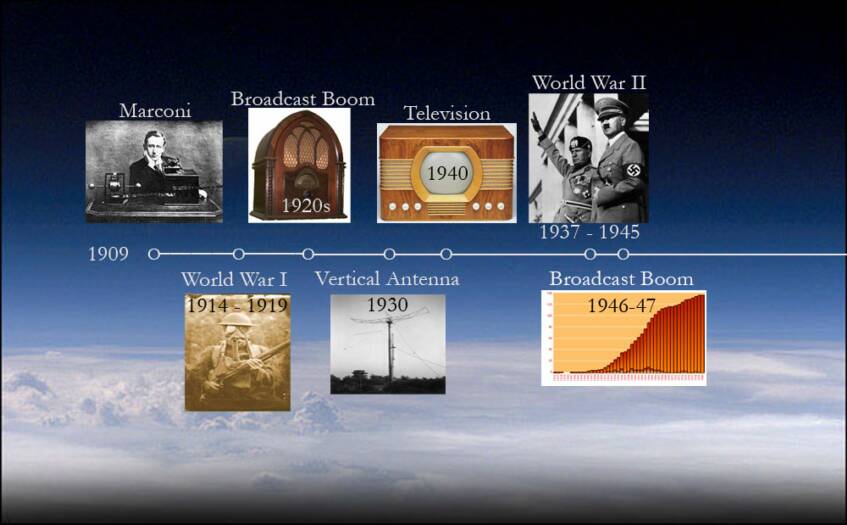
The effects of our historic broadcast on the atmosphere and the global temperature can be broken down into five time periods and four processes.

1909 The first regular broadcast over the airwaves.

1917 – 1919 WWI brought about government regulation and nearly all AM

broadcast ventures and equipment were halted and confiscated.

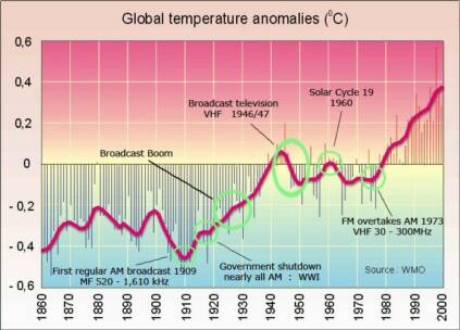
1919 – 1925 Broadcast Boom can be seen in the global temperature anomalies

graph as the REP/EEP-NOx process caused ozone depletion.

1946/47 The end of WWII brought about the largest shift in man made radio

wave propagation through the ionosphere between the US and the UK

1970’s The rise of FM and many other networks from satellite to cellular

cause an increase in electron density that allows the EEP-NOx ozone

depletion process to occur.

A rise in AM broadcast causes electron precipitation that leads to ozone depletion which causes the global temperature to rise through increased water vapor via the greenhouse effect.

The few times in history this process has been hindered can be seen in the global anomalies graph as a drop in temperature or flat spots that maintain on the 5 year mean.

Television causes a suppression of ozone depletion and the REP/EEP-NOx process and can be seen in the global temperature anomalies graph, as the temperature falls. This causes the water vapor to condense, and can be seen as peaks in historic weather events and ocean oscillations.

As FM overtook AM in the 1970’s it filled the gap between the E and F layers of the ionosphere and created a conductive bridge for the cyclotron energy to continue ozone depletion through the REP/EEP-NOx process.

1909

It is important to understand a little about the history of the broadcast industry to understand its chronological effects on the atmosphere. As we can see through the previous sections of Broadcast Theory, the AM stations that broadcast in the gyrofrequency range (630kHz ~ ((~1.45MHz)) ~ 1630kHz) excite and create plasma waves in the ionosphere leading to electron precipitation (the REP/EEP-NOx process). This leads to ozone depletion which causes the global temperature to rise through increased water vapor via the greenhouse effect. In 1909 when broadcasting first began it is hard to say that one AM broadcast station could have had much of an impact on the atmosphere. But there are a few considerations to take into account, such as the antennae design and the power necessary to transmit a receivable signal to early receivers that were of a crude design.

"The top load wire can increase radiated power by 2 to 4 times (3 to 6 dB) for a given base current." https://en.wikipedia.org/wiki/T-antenna

"ERP is equal to the input power to the antenna multiplied by the gain of the antenna." https://en.wikipedia.org/wiki/Effective_radiated_power

The first experimental antenna designs were large and complex using a ‘flattop’ antenna design, which propagates skywave far better (x2 ~ 4) than the ‘vertical’ antennas that we developed later in the 30’s. Early skywave caused radio signals to bounce back from the sky and creating a great deal of interference like heterodyne tones that magnify the effects of interference 10 times and upset broadcasters. The HAARP scientific transmitter in Alaska uses a flattop antenna design for its effectiveness in ionosphere frequency pumping and experimental excitation of plasma wave phenomena such as those seen in the REP/EEP-NOx process.

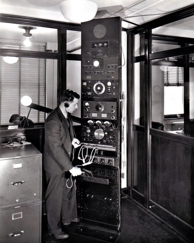
Our history of broadcast technology paints a clear picture as to the amount of power these early stations generated using powerful spark gap technology.

“huge spark stations of tremendous power were developed, using giant antennas. By later standards these early stations were absurdly overpowered – in fact they were so powerful that their signals were probably traveling around the world more than once. However receivers were so insensitive, these transmitting behemoths were needed in order to insure quality service.” (Page 86)

On Building the Broadcast Band : http://www.oldradio.com/archives/general/buildbcb.html

1917 – 1919

Perhaps these huge spark stations were too powerful because the government confiscated nearly all broadcasting and receiving equipment in 1917 after the onset of WWI, no doubt in fear that the enemy would receive news and information through these channels for tactical purposes. Westinghouse was the only civilian station allowed to continue broadcasting. During the war, the government and military experimented with spark gap technology and refined it to create vacuum tubes that were more efficient and controlled. This too could have had a profound effect on the generation of plasma waves in the ionosphere compared to spark gap technology. In 1919 when the war restrictions were lifted, the vacuum tube technology replaced the spark gap transmitters, yet however more efficient the vacuum tubes may have been, the number of stations that came over the airwaves might have easily outweighed any reduction of plasma waves in the ionosphere and the REP process due to the advancement of the technology.

During this time it is important to note the appearance of a flat spot on the global temperature anomalies graph. As I have mentioned previously flat spots are not possible in any natural cycle over such a time period of 3 years. The effects of astrophysical radio sources on ozone levels such as solar proton and cosmic rays events last no longer than 8 months as passing events. With this in mind the only source of ozone depletion that could have a longer lasting effect on this process could be from a bright broadband source of an earthly origin. Broadcasting electromagnetic energy into the ionosphere – magnetosphere mechanism is the only source that could provide constant depletion through the REP/EEP-NOx process.

1919 – 1926

The broadcast boom occurred with the world’s exciting discovery of this new technology, and can be seen in the global temperature graph. As broadcast took off, the temperature soared faster and higher. By 1920, human voice and strains of music were heard regularly over the airwaves. In 1921 there was 1 regular broadcast station and by March of 1923 there were 556 stations licensed. Radio grew explosively between 1921 and 1926, with the biggest part of the boom between 1922 and 1925. Newspapers and department stores started broadcasting and advertising. The Netherlands, Argentina and other countries followed suit as it began to spread across the globe.

It is also important to understand that pre-WW2 stations were listed by TRANSMITTER power (TPO), not ERP.

Flat top antenna was actually 2-4 times higher as ERP: 50kW TPO= 100kW ~ 200kW ERP and 150kW TPO= 300-600kW ERP

"We demonstrate that signals at 28.5 kHz emitted from the Naval (NAU) transmitter in Puerto Rico efectively couple into ionospheric ducts, induced/enhanced by the Arecibo HF heater, and propagate into the conjugate hemisphere as ducted whistlers. Also presented are suspected radar detections of whistler-triggered electron precipitation events. NAU emits VLF waves at a power and frequency of 100 kW and 28.5 kHz, respectively."

https://www.researchgate.net/publication/267719537_Whistler_Wave_I_n_teractions_with_Space_Plasmas_during_HF_Heating_of_the_Ionosphere_at_Arecibo

1946/47

The onset of WWII (1939 – 1945) brought further government experimentation and expansion to broadcasting and receiving technology. During this time control of the airwaves was still a complicated issue with many new problems arising which led to an overhaul of the broadcast system between new FM and television frequency allocations, while AM stayed the same.

Although television became commercially available in the late 30’s, it wasn’t until after the war with the FCC’s revamp of frequency allocation that television broadcasting really took off, with new television transmitters being built all over the United States. It went from four stations in 1942 to more applications than the FCC could handle in 1946 even though it allotted 400 stations in 140 metropolitan cities with a maximum power of 50kw.

Also during 1946 the UK war restrictions on broadcast lifted resulting in a television broadcast boom and caused the tropospheric ducting of UK television signals which were received around the world, that together with the US resulted in the largest frequency shift of man made radio wave propagation ever to occur in the ionosphere. This resulted in a massive electron density shift in the ionosphere and polar regions which can be seen in weather records and ocean oscillation cycles. Television operates in a frequency band that has been shown through experiments at HAARP to cause a suppression of the REP/EEP-NOx process. The effects of television on the ionosphere have already been covered in earlier chapters as well as the REP/EEP-NOx process and its effects on ozone, solar radiation, water vapor and the greenhouse effect. Refer to those sections for more information.

It is also important to understand that, both CO2 and solar activity were on the rise during the 5 years the temperature took a nose dive from 1947 - 51.

Thus ruling them out as likely causes.

“The BBC temporarily ceased transmissions on September 1, 1939 as World War II began. After the BBC channel B1 television service recommenced in 1946, distant reception reports were received from various parts of the world, including Italy, South Africa, India, the Middle East, North America and the Caribbean.” (Page 94)

“World War II research had raised issues of interference from sky waves in the 42 to 50MHz band which had been previously assigned. The catalyst for the dispute over this allocation and an advocate to move the range to higher frequencies was an FCC engineer, Kenneth Norton. During the war, he served in a capacity which made him knowledgeable of the experimental programs in the sky-wave propagation of VHF signals. He combined the War Department results with data obtained from the Bureau of Standards, and from measurements obtained on a commercial FM station, WGTR in Paxton [44.3MHz@340kW], Massachusetts, to develop new predictions of VHF sky-wave transmission. He calculated the amount of co-channel interference in the 42 to 50MHz band. He concluded that objectional interference would occur, especially in rural areas, at the extreme end of the broadcast range. Norton assumed that the broadcast signal must be ten times as strong as the interfering signal. On May 9, 1945, the FCC issued an order to raise the band for FM to 84 to 102MHz frequency range. Just two days earlier, the War Production Board announced the plan to permit the manufacturing of radio receivers. The manufacturers of the 42 to 50MHz equipment. owners of sets, and in particular Zenith, a leader in the band, had lost a profitable edge, and owned obsolete equipment. The FCC ruling also included specifications on channel widths, power, antenna height and frequency assignments. Three classes of stations were established, local stations with maximum radiated power of 50KW, regional with 50, and 100KW” (Page 92) https://www.gpo.gov/fdsys/pkg/GOVPUB-C13-4b3741bcc071ffccebb356c7673865f7/pdf/GOVPUB-C13-4b3741bcc071ffccebb356c7673865f7.pdf

1970’s

For decades, our use of television frequencies dampened the cyclotron (gyro) energy that occurred in the REP/EEP-NOx process from AM broadcast. In fact if it weren’t for the solar anomaly in 1960, with solar cycle 19, we would have likely maintained a relatively constant temperature till FM finally overtook AM in the 70’s. The golden age of radio had already given way to the top forty style broadcast of the modern era, and by this time the ionosphere was being over driven and over loaded with electrical input of electromagnetic energy from broadcast and satellite and cellular networks. The current trend in HDTV broadcast and increasing cellular and wireless networks will no doubt bring new challenges to our rising global temperatures as long as we continue to broadcast in the gyro frequency range, the source of our ozone depletion. Again the effects of FM on the environment have been discussed in earlier chapters so please refer accordingly for more information on this process.

Another space-based RF survey at 1.0–5.6 MHz measured from 100,000 to 120,000 km above Earth is reported in the work of LaBelle et al. [1989], also compared noise amplitudes with a previous survey [Herman et al., 1973] and found evidence of increasing man-made terrestrial background between 1973 and 1988.

https://pdfs.semanticscholar.org/9fb8/56bd463cbc820bb9ff553a139cd6fffb782d.pdf

Next click here

Next click here

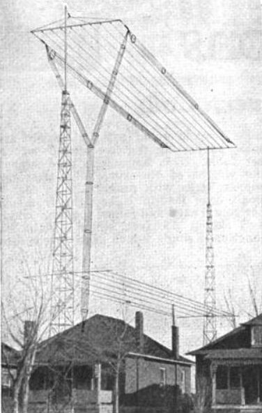
Multiwire T broadcast antenna of early AM station WBZ, Springfield, Massachusetts, 1925

http://www.theradiohistorian.org

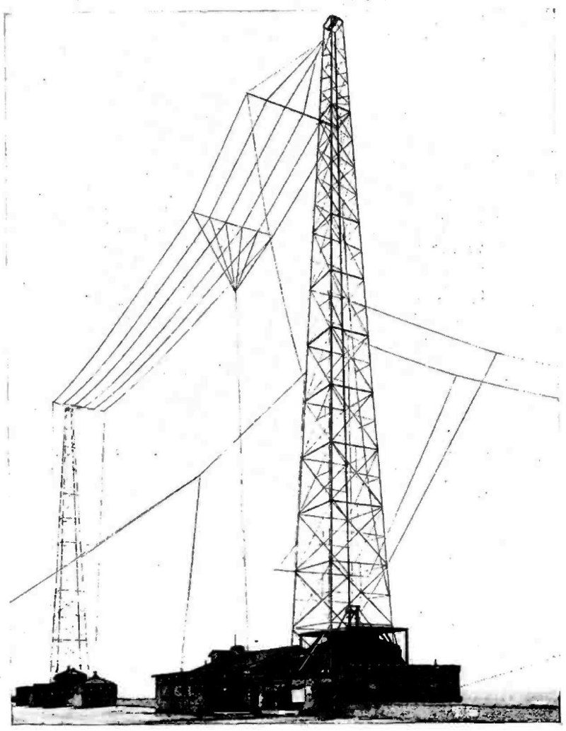
Wire radio transmitting antenna built by radio amateur William D. Reynolds, 9ZAF, of Denver, Colorado, USA around 1920, which was also the initial transmitting site for broadcasting station KLZ, first licensed March 10, 1922. It is an elaborate inverted-L antenna, which was widely used on the longwave radio bands popular during the early 20th century.

Luxembourg-Gorky Effect

Radio Luxembourg operated on 252 kHz, with a powerful 150 kw signal designed to provide coverage in England.

The phenomenon was discovered in 1933 by B.D.H. Tellegen, in Eindhoven, Netherlands, who was listening to a station in Beromunster, Switzerland, on 652 kHz.

Cross-Modulation

By beaming two signals into the ionosphere, one at 4.000000 MHz, and one at 4.0000001 MHz, the result would be a radio wave, generated in the ionosphere, with a frequency of the difference, 0.0000001 MHz, or 0.1 Hz.

Low Power Luxembourg

During a wave propagation experiment on 24 MHz in northern Sweden an unexpected phenomenon was found. This was somewhat similar to the previously known Luxembourg effect with the exception that this high frequency was used but with much lower transmitter power, 600-800 W.

Click for Source

WGY, Schenectady

GE had dabbled with radio as early as 1912 when it operated experimental station 2XI. Then, late in 1921, the company decided to construct a new broadcasting station at its manufacturing facility in Schenectady, New York. The station received the fortieth broadcasting license issued by the Department of Commerce, authorized for a power of 1,500 Watts – which at that time was the most powerful station in the country. The call letters WGY were assigned. In the early part of the 1920’s, WGY – along with most other broadcasters – shared the single frequency of 360 meters – 833 kHz.

In 1924, WGY increased its power to 5,000 watts, moving its transmitter to the current location in Rotterdam. This was G.E.’s South Schenectady transmitter laboratory, a 54 acre site which also housed the company’s two shortwave stations. Here, WGY broadcast from a 240 ft. high vertical “cage” antenna with ground radials instead of the usual T-type antenna of the time. (This antenna was replaced with the present 625 ft. half-wave tower in 1938.) Soon afterwards, the power was increased to 10,000 watts.

The Department of Commerce was interested in exploring

“super power” broadcasting, and so authorized WGY and WJZ to be the nation’s first 50 kW stations. WGY was the first station to operate at that power, more than a year ahead of WJZ, beginning its experimental high power broadcasts on July 18, 1925. Full time operation was authorized on May 8, 1926. In 1927, WGY was allowed to operate at 100 kW from midnight to 1:00 AM under a 30-day experimental license. In 1930 WGY operated for a short time experimentally at 200 kW, and received signal reports from as far away as New Zealand; but these powers were never formally approved and the station returned to 50 kW operation.

Long Distance Broadcast

In 1923, KHJ in Los Angeles picked up and rebroadcast a program received over the air from KGU in Honolulu.

In 1925, WGY in Schenectady broadcast a bridge game between players in its studio and another team 6,000 miles away in Buenos Aires.

WGY also aired a long-distance stunt in 1928 when it broadcast a three-way conversation between its studio, Australia and Java.

One of the most ambitious long-distance broadcasts took place starting in 1933, when CBS aired a weekly series of programs from the South Pole during Admiral Byrd’s expedition to Little America. To facilitate the program, CBS installed a 1,000 watt shortwave station, KFZ, at the South Pole, broadcasting from a prefabricated building that served as both a radio studio and living quarters for the staff. The KFZ programs were picked up by a high powered Argentine shortwave station and re-transmitted to the network in New York.

FCC Expands AM Band

In 1927, the FRC had decided not to expand the AM broadcast band from 1500-2000 kHz

In 1932 the FCC created three frequencies to be used by experimental wideband “high fidelity” AM stations — 1530, 1550 and 1570 kHz.

all operating at 1 kW:

W1XBS 1530 Waterbury CT

W2XR 1550 Long Island, NY

W6XAI 1550 Bakersfield, CA

W9XBY 1530 Kansas City

Ultra Short Wave - AM Apex

About the same time, experiments were begun using high fidelity AM transmissions at what was then considered the upper limits of practical radio technology. Those frequencies, between 25 and 42 MHz, were called “Ultra Short Wave.”

These radio stations were called “Apex” stations because of their high frequencies and high antenna locations.

They could operate up to 1,000 watts on several groups of frequencies at 25-26 MHz and 42 MHz

By 1939, there were Apex station stations operating in 34 cities in 22 states.

As today’s ten meter ham radio operators know very well, propagation conditions on the frequencies that were used by the Apex stations vary tremendously over the eleven year sunspot cycle.

The sun was just coming out of a sunspot minimum when the first Apex experiments began in 1932, so the new stations probably experienced mostly interference-free coverage during their first few years of operation. But sunspots were at their peak in 1936, and suddenly the experimental Apex stations were being heard all around the globe.

W9XAZ in Milwaukee reported that its signal was stronger in Los Angeles than was the local station.

FCC Shuts off AM Apex

In its 1941 announcement, the FCC also announced that it would terminate all existing experimental high frequency licenses, both AM and FM, on January 1, 1941, and encouraged those stations to reapply for new commercial FM licenses. No AM broadcasting on the ultra-high frequencies would now be allowed. The Apex stations began shutting down or converting to FM in droves.

WTMJ-FM 1948 Super FM

92.3MHz @ 349kW

WW2 Mid 40's Discovers Ionospheric Turbulence on LW FM 42MHz

WGTR - 44.3MHz @ 340kW

(Sporadic E interference)

Sporadic E: Artificial Traveling Ionospheric Disturbances

RADAR OBSERVATIONS OF ARTIFICIAL IONOSPHERIC TURBULENCE DURING A MAGNETIC STORM

Notes:

AM Apex frequency

25-26MHz & 42MHz

1,000 Watts TPO

2,000~4,000 Watts ERP

Low Power Luxembourg

24MHz @ 600-800watts

FCC Apex Shutdown

1932 - 1941

Could the temperature rise during this period on WMO temp graph be attributed to Apex - Transmitter Induced EEP-NOx specifically in an atmosphere that had never been subjected to these frequencies before?

When FCC shut down Apex, the global temperature dropped for nearly 5 years.

Next click here

WWII - Bureau of Standards Report: Ionospheric Turbulence on Long Wave FM

Radio waves from Earth clear out space radiation belt 9 June 2008

Naval Communication Station Harold E. Holt is located on the northwest coast of Australia, 6 kilometres (4 mi) north of the town of Exmouth, Western Australia.

Interestingly, the new work suggests researchers have never observed the Van Allen belts as they are “naturally”. That’s because VLF radio transmitters have been used since at least the 1920s to send telegraph messages and communicate with submarines, and the belts’ existence was only confirmed in 1958.

“Electron lifetime [in the belts] now must be different than it was before the transmitters were built, but we don’t know how different,” Rodger told New Scientist.

https://www.newscientist.com/article/dn14089-radio-waves-from-earth-clear-out-space-radiation-belt/

Television Growth

Television Start

https://www.youtube.com/playlist?list=PL18A480E27C4EDD07

This element is no longer available.

The Van Allen Radiation Belt: U.S. Historical Perspective ~ 2018

https://vimeo.com/254023376

WLW Super power Station 500kW

In January 1934, WLW began broadcasting with 500,000 watts after midnight under the experimental call sign W8XO. In April 1934 the station was authorized to operate at 500,000 watts during regular hours using the WLW call letters. On May 2, 1934, President Franklin D. Roosevelt ceremonially pressed the same golden telegraph key that Wilson had used to open the Panama Canal, officially launching WLW's 500-kilowatt signal.[36]

As the first station in the world to broadcast at this strength, WLW received numerous complaints from around the United States and Canada that it was interfering with other stations, most importantly from CFRB, then on 690 kHz, in Toronto, Ontario. In December 1934, WLW was instructed to cut back to 50 kilowatts at night until it had eliminated the interference.[37] The station began construction of two shorter towers 1850 feet (560 m) southwest from the main tower in order to create a directional antenna, which successfully reduced the signal broadcast towards Canada. With these antenna towers in place, full-time broadcasting at 500 kilowatts resumed in early 1935. However, WLW was continuing to operate under special temporary authority that had to be renewed every six months; each renewal brought complaints about interference, and undue domination of the market, by such a high-power station.

On March 1, 1939, WLW resumed operations at 50,000 watts.[47] The station had unsuccessfully attempted to reverse the decision in the courts, and now had to shut down the huge amplifiers, except for brief, experimental night periods as W8XO.[48] Because of the impending war, and the possible need for national broadcasting in an emergency, the W8XO experimental license for 500 kilowatts remained in effect until December 29, 1942.